Monday, March 9, 2009

Principle Component Analysis in Python


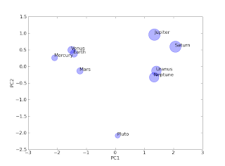
While there a number of tutorials and pages better devoted to the subject of principle component analysis (PCA), this post is geared towards providing a simple example of this data classification method in python. Much of the algorithm code was provided by Henning Risvik. This module along with numpy, scipy, and matplotlib are required for this example to function. The data used for this example are derived from the physical properties of the planets (the debate over Pluto's status is for another post but is assumed to retain it's planet privileges for this post). The pca module required for this example can be found here.


'''
PCA example using python. Very simplified
'''

import pca_module as pca
import numpy as N
import pylab as P
'''
Adapted from:

http://www.cs.mcgill.ca/~sqrt/dimr/dimreduction.html

[title] Planets of the Solar System
[source] http://pds.jpl.nasa.gov/planets/

[columns] distance diameter density
"Mercury" 0.387 4878 5.42 (black)
"Venus" 0.723 12104 5.25 (black)
"Earth" 1.000 12756 5.52 (black)
"Mars" 1.524 6787 3.94 (black)
"Jupiter" 5.203 142800 1.314 (blue)
"Saturn" 9.539 120660 0.69 (blue)
"Uranus" 19.18 51118 1.29 (blue)
"Neptune" 30.06 49528 1.64 (blue)
"Pluto" 39.53 2300 2.03 (blue)

'''
RawPlanets = N.array([
[0.39,4878,5.42],
[0.72,12104,5.25],
[1,12756,5.52],
[1.52,6787,3.94],
[5.2,142800,1.31],
[9.54,120660,0.69],
[19.18,51118,1.29],
[30.06,49528,1.64],
[39.53,2300,2.03]])

#Normalize the raw values
dataMatrix = N.log10(RawPlanets)

#perform PCA--thanks Henning Risvik
scores, loading, explanation = pca.PCA_nipals2(dataMatrix, standardize=True)

pc1 = scores[:, 0]
pc2 = scores[:, 1]
pc3 = scores[:, 2]

fig=P.figure()#create pylab figure
ax = fig.add_subplot(111)#create an ax

#add scatter plot and size based upon distance from sun
ax.scatter(pc1, pc2, color = 'b', s = dataMatrix[:,1]**4, alpha = 0.3)

#add axis labels
ax.set_xlabel('PC1', fontsize = 12)
ax.set_ylabel('PC2', fontsize = 12)

#data labels
labels = ['Mercury','Venus', 'Earth', 'Mars', 'Jupiter', 'Saturn', 'Uranus', 'Neptune', 'Pluto']
#add labels to each marker
for label, x, y in map(None, labels, pc1, pc2):
ax.annotate(label, xy=(x, y), size = 12)

P.show()

Thursday, January 8, 2009

Slow Mo Bubble Burst


This is an amazing video detailing the slow motion video capture of a bubble bursting. While it does not seem like much, it can be terribly fascinating. Fast forward to just under 4:00 for the slow motion capture.

Fitting an Arbitrary Function in Python


While peak areas may be measured directly through trapezoidal integration, in some cases the true analytical signal is convoluted with some degree of noise (whether that noise is stochastic or systematic is another matter). One solution minimize the contribution of noise to a particular signal is through fitting. While fitting a least squares line can be easily achieved using a simple scientific calculator, the fitting of more complex functions is, you guessed it, more complex. Not only is the function itself more involved than a straight line, the fitting methods used often require a initial fitting parameters to start. Often these are educated guesses regarding the nature of the data you are trying to fit. Below is an example of fitting both a gaussian and exponentially modified gaussian functions (common chromatographic peak shapes) to hypothetical data. Perhaps the two most salient features in the code snippet below are the use of the FFT to convolute two different functions to create the EMG and the use of a fairly generic syntax which accepts a variable number of parameters and an arbitrary function to fit the data. This code snippet was highly influence by the information already posted on the scipy website regarding function fitting.

The next task...how to tell the difference between the fitted function and the actual data? Any takers?

I should also note that another good example can be found here.


import numpy as N
import numpy.fft.fftpack as F
'''

Next how to calculate area?
'''

def expGauss(x, pos, wid, tConst, expMod = 0.5, amp = 1):
'''
x -- numpy array
pos -- centroid position
wid -- width
tConst -- time constance for exponential decay
amp -- amplitude of peak
expMod -- modifies the amplitude of the peak -- must be a float

Forumulas used:

y = a * exp(-0.5 * (x-b)^2 / c^2) --traditional gaussian forumla
exp = N.exp(-1*expMod*N.arange(0,len(y))/Const) --function that is merged with the gaussian

Note if expMod is too small (i.e. goes towards zero) the function will return a flat line.
'''
expMod *=1.0
gNorm = amp * N.exp(-0.5*((x-pos)/(wid))**2)
g = expBroaden(gNorm, tConst, expMod)
return g, gNorm

def expBroaden(y, t, expMod):
fy = F.fft(y)
a = N.exp(-1*expMod*N.arange(0,len(y))/t)
fa = F.fft(a)
fy1 = fy*fa
yb = (F.ifft(fy1).real)/N.sum(a)
return yb

if __name__ == '__main__':
import scipy as S
import pylab as P
import scipy.optimize as optimize

a = N.arange(0,100,0.1)

tConstArray = N.arange(10,200,10)
x, x1 = expGauss(a, 50, 2, 150, 2, 5)
xN = x + 0.5-S.rand(len(a))/2
x1N = x1 + 0.5-S.rand(len(a))/2


# Fit the first set
#p[0] -- amplitude, p[1] -- position, p[2] -- width
fitfuncG = lambda p, x: p[0]*N.exp(-0.5*(x-p[1])**2/p[2]**2) # Target function
errfuncG = lambda p, x, y: fitfuncG(p, x) - y # Distance to the target function
p0 = [5.0, 50.0, 2.0] # Initial guess for the parameters
p1, success = optimize.leastsq(errfuncG, p0[:], args=(a, x1N))
p1G = fitfuncG(p1,a)

P.plot(x1N, 'ro', alpha = 0.4, label = "Gaussian")
P.plot(p1G, label = 'G-Fit')

'def expGauss(x, pos, wid, tConst, expMod = 0.5, amp = 1):'
#p[0] -- amplitude, p[1] -- position, p[2] -- width, p[3]--tConst, p[4] -- expMod
fitfuncExpG = lambda p, x: expGauss(x, p[1], p[2], p[3], p[4], p[0])[0]
errfuncExpG = lambda p, x, y: fitfuncExpG(p, x) - y # Distance to the target function
p0a = [3.5, 45., 3., 70., 2.] # Initial guess for the parameters
p1a, success = optimize.leastsq(errfuncExpG, p0a[:], args=(a, xN))
p1aG = fitfuncExpG(p1a,a)

print type(xN), type(a), len(xN), len(a)
P.plot(xN, 'go', alpha = 0.4, label = "ExpGaussian")
P.plot(p1aG, label = 'ExpG-Fit')

P.legend()
P.show()